Class VIII

If

Simple If Examples | And/Or Criteria | Nested If

The IF function is one of the most used functions in Excel. This page contains many easy to follow IF examples.

Simple If Examples

The IF function checks whether a condition is met, and returns one value if true and another value if false.

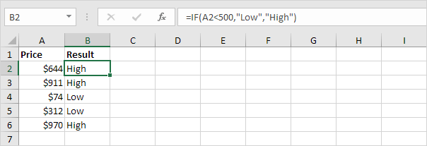
1a. For example, take a look at the IF function in cell B2 below.

Explanation: if the price is greater than 500, the IF function returns High, else it returns Low.

1b. The following IF function produces the exact same result.

Note: you can use the following comparison operators: = (equal to), > (greater than), < (less than), >= (greater than or equal to), <= (less than or equal to) and <> (not equal to).

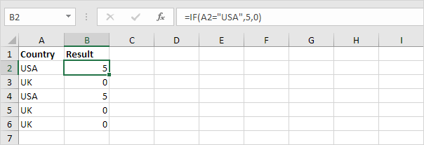
2. Always enclose text in double quotation marks.

3a. The formula below calculates the progress between two points in time.

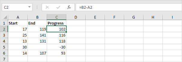
3b. You can use the IF function to display an empty string ("") if the end value hasn't been entered yet (see row 5).

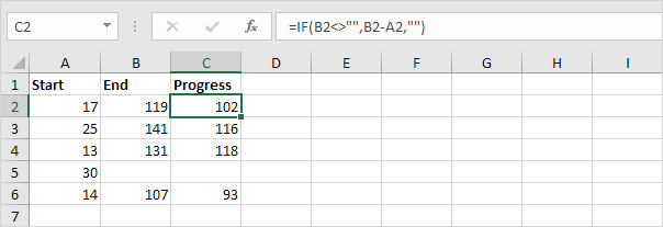
Explanation: if the end value is not empty (<> means not equal to), the IF function calculates the progress between the start and end value, else it displays an empty string ("").

And/Or Criteria

Use the IF function in combination with the AND function and the OR function and become an Excel expert.

1. For example, take a look at the IF function in cell D2 below.

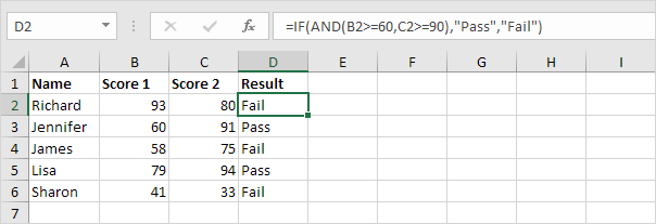
Explanation: the AND function returns TRUE if the first score is greater than or equal to 60 and the second score is greater than or equal to 90, else it returns FALSE. If TRUE, the IF function returns Pass, if FALSE, the IF function returns Fail.

2. For example, take a look at the IF function in cell D2 below.

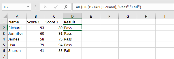
Explanation: the OR function returns TRUE if at least one score is greater than or equal to 60, else it returns FALSE. If TRUE, the IF function returns Pass, if FALSE, the IF function returns Fail.

3. For example, take a look at the IF function in cell D2 below.

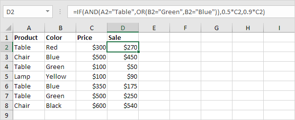
Explanation: the AND function has two arguments (table, green or blue). The IF function reduces the price of green and blue tables by 50% and reduces the price of all other products by 10%.

Nested If

The IF function in Excel can be nested, when you have multiple conditions to meet. The FALSE value is being replaced by another IF function to make a further test.

1. For example, take a look at the nested IF formula in cell C2 below.

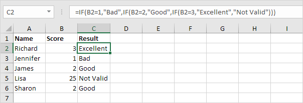
Explanation: if the score equals 1, the nested IF formula returns Bad, if the score equals 2, the nested IF formula returns Good, if the score equals 3, the nested IF formula returns Excellent, else it returns Not Valid. If you have Excel 2016, simply use the IFS function.

2. For example, take a look at the nested IF formula in cell C2 below.

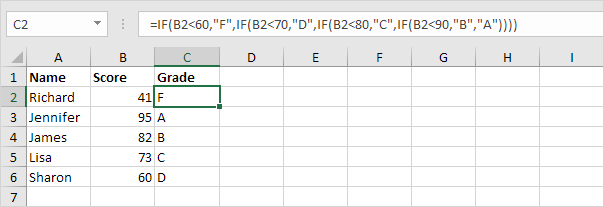
Explanation: if the score is less than 60, the nested IF formula returns F, if the score is greater than or equal to 60 and less than 70, the formula returns D, if the score is greater than or equal to 70 and less than 80, the formula returns C, if the score is greater than or equal to 80 and less than 90, the formula returns B, else it returns A.

Make Nested if in given below data Score	Grade
0-63	F
64-72	D
73-84	C
85-94	B
95-100	A

Basics of Spreadsheet

A spreadsheet -> is a large sheet having data and information arranged in rows and columns. As you know, Excel is one of the most widely used spreadsheet applications. It is a part of Microsoft Office suite. Spreadsheet is quite useful in entering, editing, analyzing and storing data. Arithmetic operations with numerical data such as addition, subtraction, multiplication and division can be done using Excel. You can sort numbers/ characters according to some given criteria (like ascending, descending etc.) and use simple financial, mathematical and statistical formulas. 

Importance of Microsoft Excel for Students

1 In Excel, students can do and learn the fastest way to do calculation with accuracy. 

2. Microsoft Excel builds strong analytical thinking and skills

3. Students can learn how calculation are performed

4. Students can learn how data is visualized

FEATURES OF SPREADSHEETS There are a number of features that are available in Excel to make your task easier. Some of the main features are:

 1. AutoSum - helps you to add the contents of a cluster of adjacent cells. 

2. List AutoFill - automatically extends cell formatting when a new item is added to the end of a list. 
3. AutoFill - allows you to quickly fill cells with repetitive or sequential data such as chronological dates or numbers, and repeated text. AutoFill can also be used to copy functions. You can also alter text and numbers with this feature. 

4. AutoShapes toolbar will allow you to draw a number of geometrical shapes, arrows, flowchart elements, stars and more. With these shapes you can draw your own graphs. 

5. Wizard - guides you to work effectively while you work by displaying various helpful tips and techniques based on what you are doing. 

6. Drag and Drop - it will help you to reposition the data and text by simply dragging the data with the help of mouse. 

7. Charts - it will help you in presenting a graphical representation of your data in the form of Pie, Bar, Line charts and more.

 8. PivotTable - it flips and sums data in seconds and allows you to perform data analysis and generating reports like periodic financial statements, statistical reports, etc. You can also analyse complex data relationships graphically.

 9. Shortcut Menus - the commands that are appropriate to the task that you are doing will appear by clicking the right mouse button.

STARTING EXCEL 
1. Click on (with the help of mouse) the Window button on the  at the bottom of the Screen 
2. Highlight the Programs item. The program menu will open. 
3. Select Microsoft Excel from the list of programs. 
 4. Click on Microsoft Excel Symbolically these actions are shown below.

 Select Window Button→Programs→Microsoft Excel commands from your menu bar.

EXCEL WORKSHEET Excel allows you to create worksheets much like paper ledgers that can perform automatic calculations. Each Excel file is a workbook that can hold many worksheets. The worksheet is a grid of columns (designated by letters) and rows (designated by Microsoft Excel MSOB Basics of MS Excel :: 229 numbers). The letters and numbers of the columns and rows (called labels) are displayed in gray buttons across the top and left side of the worksheet. The intersection of a column and a row is called a cell. Each cell on the spreadsheet has a cell address that is the column letter and the row number. Cells can contain either text, numbers, or mathematical formulas

12.5.1 Selecting, Adding and Renaming Worksheets 
The worksheets in a workbook are accessible by clicking the worksheet tabs just above the status bar. By default, three worksheets are included in each workbook. To add a sheet, select Insert→Worksheet from the menu bar. To rename the worksheet tab, move the cursor to sheet tab, right-click on the tab with the mouse and select Rename from the shortcut menu. Type the new name and press the ENTER key


12.7 NAVIGATING THE WORKSHEET You can advance through your worksheet by rows with the vertical scrollbar or by columns with the horizontal scrollbar (see Figure 13.2). when you click and drag the thumb tab on the scrollbar, a Screen Tip will appear alongside the bar identifying the row or column to which your view is advancing. You can also use keyboard shortcuts given at the end of this lesson for navigating the worksheet


12.8 DATA ENTRY You can enter various kinds of data in a cell. 
1. Numbers: Your numbers can be from the entire range of numeric values: whole numbers (example, 25), decimals (example, 25.67) and scientific notation (example, 0.2567E+2). Excel displays scientific notation automatically if you enter a number that is too long to be viewed in its entirety in a cell. You may also see number signs (# # # # # #) when a cell entry is too long. Widening the column that contains the cell with the above signs will allow you to read the number.

2. Text: First select the cell in which data has to be entered and type the text. Press ENTER key to finish your text entry. The text will be displayed in the active cell as well as in the Formula bar. If you have numbers to be treated as text use an apostrophe (‘) as the first character. You cannot do calculations with these kind of data entry.

 3. Date and Time: When you enter dates and times, Excel converts these entries into serial numbers and kept as background information. However, the dates and times will be displayed to you on the worksheet in a format opted by you. You will learn about date and time formats later in lesson 10. 

4. Data in Series: You can fill a range of cells either with the same value or with a series of values with the help of AutoFill.


12.9 EDITING DATA Editing your Excel worksheet data is very easy. You can edit your data by any of the following ways: 
1. Select the cell containing data to be edited. Press F2. Use Backspace key and erase the wrong entry. Retype the correct entry. 
2. Select the cell and simply retype the correct entry. 
3. If you want only to clear the contents of the cell, select the cell and press Delete key.
 4. To bring back the previous entry, either click on Undo button on standard Toolbar or select Edit→Undo command or use keyboard shortcuts CTRL+Z

12.12 MODIFYING A WORKSHEET 12.12.1 Adding Rows, and Columns 1. Worksheets - 
 1. Row - To add a row to a worksheet, select Insert→Rows from the menu bar, or highlight the row by clicking on the row label, right-click with the mouse, and choose Insert. 
2. Column - Add a column by selecting Insert→Columns from the menu bar, or highlight the column by click on the column label, right-click with the mouse, and choose Insert.

12.12.2 Resizing Rows and Columns There are two ways to resize rows and columns.
 1. Resize a row by dragging the line below the label of the row you would like to resize. Resize a column in a similar manner by dragging the line to the right of the label corresponding to the column you want to resize. 
2. Click the row or column label and select Format→Row→Height or Format→Column→Width from the menu bar to enter a numerical value for the height of the row or width of the column.

12.12.3 Selecting Cells 
Before a cell can be modified or formatted, it must first be selected (highlighted). Refer to the table below for selecting groups of cells. Cells to select Mouse action: 
1 One cell -click once in the cell
2 Entire row click the row label 
3  Entire column click the column label 
4   Entire worksheet click the whole sheet button (at the intersection of rows and columns) 
5 Cluster of cells drag mouse over the cells or hold down the SHIFT key while using the arrow keys

12.12.4 Moving and Copying Cells 
1. Moving Cells To cut cell contents that will be moved to another cell select Edit→Cut from the menu bar or click the Cut button on the standard toolbar. 
2. Copying Cells To copy the cell contents, select Home→Copy from the menu bar or click the Copy button on the standard toolbar. 
3. Pasting Cut and Copied Cells Highlight the cell you want to paste the cut or copied content into and select Home→Paste from the menu bar or click the Paste button on the standard toolbar.
4. Drag and Drop If you are moving the cell contents only a short distance, the drag-and-drop method may be easier. Simply drag the highlighted border of the selected cell to the destination cell with the mouse. 
5. Freeze Panes If you have a large worksheet with column and row headings, those headings will disappear as the worksheet is scrolled. By using the Freeze Panes feature, the headings can be visible at all times. 
       1. Click the label of the row below the row that should remain frozen at the top of the worksheet. 
       2. Select Window→Freeze Panes from the menu bar. 3. To remove the frozen panes, select Window→Unfreeze Panes.

Header/Footer tab gives you the option to set the Header (which will be displayed on the top of every page) and the Footer (which will be displayed on the bottom of every page). Add preset headers and footers to the page by clicking the drop-down menus under the Header/Footer tab.

 FILE CLOSE AND EXIT EXCEL 
When your work is finished and it has been saved properly:
 1. Select Office Button→Close command and then click mouse to close your file
 2. Select Office Button→Exit command and then click mouse to close your file

WORKBOOK PROTECTION You have learned how to save your workbook as a file. Some times your data can be very confidential which you would like to protect from unauthorised people. Protection prevents changes to all or part of a document. You can also assign a password so that other users can be limited in accessing protected information. A password is case sensitive, can be up to 255 characters long, and can contain any combination of letters, numbers, and symbols. When a document is protected, this command changes to Unprotect Document. You can restrict access to your workbook in three ways.

 1. Protect Sheet: Select Review→Protect Sheet commands and click. This feature prevents changes to cells on worksheets, items in a chart, graphic objects on a worksheet or chart sheet. When the active document is protected, the command name changes to Unprotect Sheet. If you want to unprotect a sheet that has been already protected. Select Tools→Unprotect Sheet commands and click. 

2. Protect Workbook: Select Review →Protect Workbook commands and click. This feature protects a workbook’s structure and windows. You can prevent changes to the structure of a workbook so that sheets can’t be deleted, moved, hidden, unhidden, or renamed, and new sheets can’t be inserted. You can also protect windows from being moved or resized. When the active document is protected, the command name changes to Unprotect Workbook. If you want to unprotect a workbook that has been already protected. Select Review→Unprotect Workbook commands and click

3. Protect for Sharing: Select Review→Protect and Share Workbook commands and click. This feature protects the sharing and change history tracking in a shared workbook so the features can’t be turned off. If you select this check box and click OK when the workbook isn’t a shared workbook, you are asked if you want to save it as a shared workbook. In a workbook that is already shared, you can turn on protection for sharing and the change history, but you can’t assign a password for this protection. To assign a password, you must first remove the workbook from shared use. When the active shared workbook is protected, the command name changes to Unprotect for Sharing. If you want to unprotect a share workbook that has been already protected. Select Review→Unprotect Workbook commands and click. 

PRINT To print the worksheet, select Office Button→Print from the menu bar.
1. Print Range - Select either all pages or a range of pages to print. 
2. Print What - Select selection of cells highlighted on the worksheet, the active worksheet, or all the worksheets in the entire workbook.
3. Copies - Choose the number of copies that should be printed. Check the Collate box if the pages should remain in order. 
4. Click OK to print